i want to keep my data for my entire life. modern hardware should be advanced enough to support this, but the real world invariably rears its ugly head whenever discussions of "forever" come up, anywhere. nothing is forever. \(P[\text{the world ends tomorrow}] > 0\), after all. my entire life (and possibly the lives of another generation or two) should be sufficient for my purposes.
note: this is a redone version of an analysis that i did for work a while
back. i was operating ~200 TB of networked storage at the time for both
background
i'm building a
not just a
this necessitates redundancy: i can't rely on a single storage device because it
will fail (\(P \approx 1\)) in 50 years. because i'm impatient (and i've done a
similar analysis before), i decided to go ahead and order four 8 TB drives, then
write this post.
if you're from the future, hello! this was in 2026, when
all i need to do is figure out, for the most reliable architecture i can build, just how reliable it really is.
architecture
my planned architecture for the
- set up the four drives in two groups of two, each
btrfsraid 1, - store one group at my father's house several states away, and
- automatically synchronize the local copy with the remote copy.
really important note if you're doing this yourself: use
the nice thing about btrfs
as well as zfs, if that's more your speed. next-gen filesystems
generally have this as a feature, because we've all started to accept that
storage is fallible and data on a computer matters to us.
for this is that it checksums each data block
(which appear to be 16 KiB per the docs) and will auto-repair corrupt blocks on
read, so long as there is a good copy of that block somewhere! this means that
if we have drives in
smart monitoring & failure policy
i'd be a fool to ignore the built-in monitoring systems that the drives have if
i care about redundancy, so: in the event of a btrfs replace with -r is the way to do this from
where your bits go when they die
there are two well, there are at least two ways hard drives can make you sad. i'm not claiming omniscience. ways hard drives can make you sad:
- they can die, or
- they can forget what you told them.
if a drive dies, you lose everything it held. the only option is to replace it
and rebuild that data from redundant copies (which you hopefully have). if a
drive has an error on read, you lose all data in that disk sector (typically 512
B). this is known in the literature as a latent sector error, or
to figure out the appropriate mathematical model for \(P[data loss]\), we have to understand the shape of these two failure modes. on to reading!
disk failure
when people talk about reliability engineering (read: equipment failure at large enough scale that you measure via statistics), they speak of the "bathtub curve:"
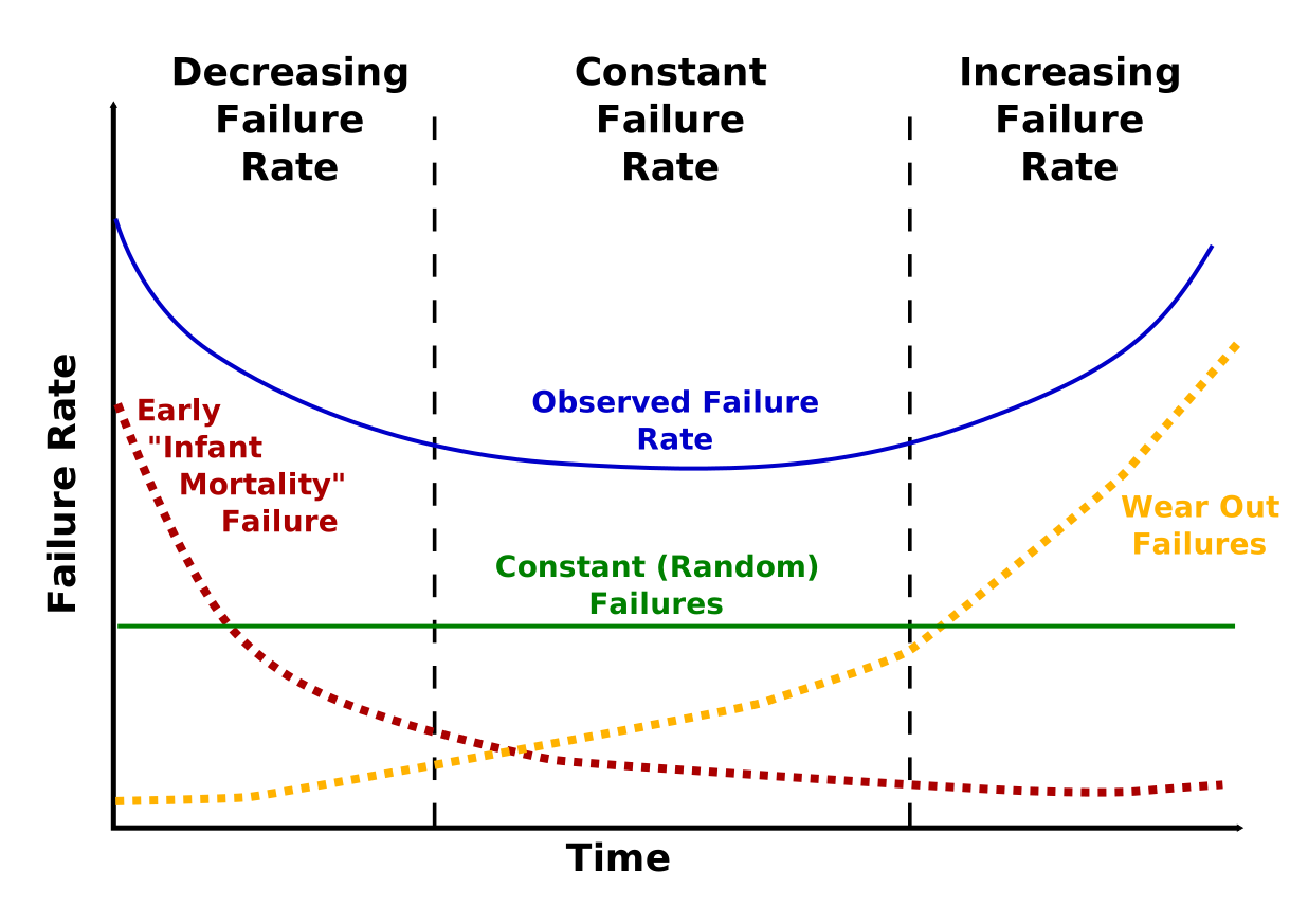
the idea is that most hardware failure is due to either manufacturing/
of course, humans aren't known for staying within datasheet
specifications… but as it turns out, neither are hard drives.
this curve is becoming increasingly less correct for modern hard drives. it was accurate-ish in the aughts, but backblaze's october 2025 post on annualized failure rates gives this graph, which is notably not a bathtub:
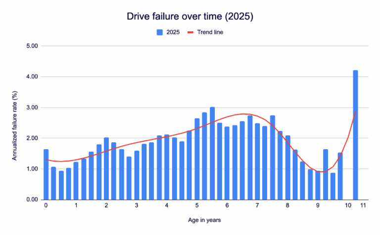
backblaze interprets this changing curve shape to mean that hard drives
reliability has improved over the past decade or so, as well as to mean that the
nature of failure has changed: annual failure rates (
that variability worries me: it indicates that true
sector failure
let's look at the other way you can lose data: a sector goes bad.
bairavasundaram et. al.'s analysis (published in sigmetrics in 2007) details
what the single-sector failure situation looked like in, well, 2007.
they observed that the conditional probability of an
according to schroeder, damouras, & gill,
in summary, if we have one
my drives specifically
annoyingly, none of these analyses seem to yield information on "how accurate are the datasheet specs relative to reality." it seems to me that the best way to determine the prior odds of either disk or sector failure is simply to take some recent data and estimate, so i'll do that.
i'm using seagate
since i didn't find a whole lot of recent failure probabilities — or ways to
describe them — in the literature, i had opus 4.7 pull the most recent
backblaze dataset (2025, as of this writing) and examine drive models similar to
the one i would be using.
opus and i had a lot of back-and-forth about what
exactly to look at in the data — we eventually settled on new
3–5% of the drives had a new
| sector count | probability |
|---|---|
| 6–20 | 81% |
| 21-100 | 15% |
| 101-500 | 2.5% |
| 500+ | 1.5% |
opus noted that the most common occurrence was an 8-sector failure, which it
theorized corresponded to a single 4 KiB on-disk sector. this seems like a
reasonable explanation, but i don't really care about the mechanics. i have a
bucketed
workload estimation
i don't really need this for the analysis i'm doing, but if i ever want to calculate my data loss expectation, i will, so i'll leave it here.
my workload consists of storing my own stuff, listening to music, and watching the occasional film. let's see:
- my home diretory uses 100 GB on this machine, and i'd like to run nightly backups, each of which might change an average of 1 GB of data (maybe, we're going conservative here);
- large film files are around 100 GB and i might watch one or two of those a week; and
- lossless spotify streaming is apparently equivalent to a 24-bit 44.1 kHz
flac , and my last wrapped indicated i listened to in neighborhood of 50 kilominutes per year of music.
most of my rate estimates here are in the units of years, which means i will read about
1 GB/day + 100 GB/month + (24 bit * 44.1 kHz * 50 kmin)/year to bit/year
1.56972E13 bits/a_j
1.5 × 1013 bits per year. also, i have a partner. call it 3 × 1013 bits per year.
on bitrot & scrubbing
many sources state that you should scrub NASes, particularly checksummed ones,
so that any bad sectors will be caught and corrected before you have to
resilver.
something i find funny about scrubbing: if you look only at the
datasheet for a hard drive, it gives a
i have found conflicting reports as to whether bitrot is a significant
occurrence on modern magnetic media. the australian government alleges that
temperature fluctuation is important, but they mostly talk about magnetic tapes.
do we know how fast — or by what mechanism — data on modern magnetic hard
disks decays? (if you know, email me!) without this knowledge, scrubbing has
unspecified efficacy, as it really only matters if the data has some nonzero
chance of changing once laid down.
one thing that's sitting in the back of
my mind here is that
however! what regular scrubbing can ensure is that, should you lose a disk
in the array, the other \(N - 1\) drives are known to have had at least one
successful read from all the lost sectors. given that schroeder et al. noted
that
i don't really know what the best policy here is, frankly, aside from inter-disk
redundancy. if there are errors, though, i'd rather know about them sooner
rather than later. readback immediately after writing, along with a periodic
(monthly, say) scrub of the entire
theory
now that i have a
\(P[\text{we lose anything at all}]\)
given our two failure modes of whole-disk failure or single-sector failure, (and
given a
- a single drive fails, and when we go to rebuild, the remaining drives experience data loss, or
- all
n drives develop anlse in the same sector at some point.
the second case covers an auto-repair failure: if every drive has an
i will assume that a given array will only experience data loss once: after the first moment of loss, the array is toast and we have to rebuild it. since failure rates, as discussed above, are relatively constant with drive age these days, i will ignore drive age completely. it also stands to reason that events on different physical drives are more or less independent, so \(P[A \cap B] = P[A]\ P[B]\). finally, though these probabilities don't depend on drive age, they do depend on the working life of the array: we really want to know \(P[\text{data loss with}\ N\ \text{drives over a lifespan}\ L]\). thus,
\begin{equation} \begin{split} & P[\text{we lose anything at all}] \\[1em] & P[\text{data loss}\ (N, T)] \\[1em] & = P[\text{one drive of}\ N\ \text{fails in}\ T \cap\ \text{data loss}\ (N - 1, R) \\[1em] & \qquad \cup\ N\ \text{drives develop the same LSE in}\ T] \\ \end{split} \end{equation}
where \(R\) denotes the time it takes us to perform a resilver (say two
weeks
this is not crazy; i figure most of the time spent responding to a
failure will be in procuring a new drive, not the actual resilver, and time is
what matters here!
) and \(N > 0\). note that \(P[\text{data loss}](N = 0, \_) = 1\),
because zero drives cannot hold any data whatsoever.
unless you're tom7, of course.
this means we need to
work out only two probabilities to get the failure chance for this
- \(P[\text{one drive of}\ k\ \text{fails in}\ t]\) and
- \(P[k\ \text{drives develop the same LSE in}\ t]\).
\(P[\text{one drive of}\ k\ \text{fails in}\ t]\)
the probability of any single drive failing is dependent on its
since
since we want to know the probability that a drive survives for \(t\) years, we
need to know how likely it is that the drive's eventual failure will come after
\(t\) years have passed. the time-to-first-event probability of a Poisson
process is given by the exponential distribution, which has
to figure out the probability we want, we just integrate this over the time range we're interested in — in this case, everything after \(t\):
\begin{equation} \begin{split} & P[\text{a drive lives for}\ t] \\ & = \int_t^\infty \lambda e^{-\lambda t}\ dt \\ & = \left.-e^{-\lambda t}\right|_t^\infty \\ & = -e^{-\infty} + e^{-\lambda t} \\ & = e^{-\lambda t} \\ & = \exp\left(-\text{AFR} \cdot t\right) \\ \end{split} \end{equation}all together, we have
\begin{equation} \label{9458878c7de3cec957e0d4fc9a465e2e} \begin{split} & P[\text{one drive of}\ k\ \text{fails in}\ t] \\ & = 1 - \exp\left(-\text{AFR} \cdot t\right)^k \\ & = 1 - \exp\left(-\text{AFR} \cdot k \cdot t\right) \\ \end{split} \end{equation}
you may recall we plan on using \eqref{9458878c7de3cec957e0d4fc9a465e2e} to describe failure
over both the working life of the
\(P[k\ \text{drives develop the same LSE in}\ t]\)
this one's more interesting, because
with, if
that last probability in \eqref{1411fb31d54e13e11aea72b812891307}, \(P[\text{the
rest share}\ \geq 1\ \text{of the}\ m]\), is the tricky one. because those \(m\)
i claim that this is hard to think about.
the thing that stymied me for a while in this analysis was: i wanted to get an
estimate of the probability of a given
so: how do we get \(P[S], S \subset D\) from \(P[s], P[s_1 | s_2], \forall s, s_1, s_2 \in D\ \)?
…you can't. i spent a while trying to do this before realizing it had some
real similarity to the problem of reconstructing the full
since there's massive uncertainty about even the quantities i would take as givens for that problem, i figured my best bet was to come up with a justifiable approach to the whole thing and run with it.
i decided i would figure that the empirical prior probability of
i will also use a real useful bit of the earlier analysis: since most btrfs blocks are 16 KiB
large, i can do the analysis with a sector granularity of 16 KiB and come much
closer to correct! a 16 KiB block is 32 × 512 B sectors, which (given the
| 16 KiB sector count | probability |
|---|---|
| 1 | 81% |
| 2–3 | 15% |
| 4+ | 4% |
now the math. for each bad sector on the drive that had a failure, we want to know the probability that, for at least one of those sectors, all the remaining drives have also failed on that sector:
\begin{equation} \begin{split} & P[\text{the rest share}\ \geq 1\ \text{of the}\ m] \\ & = P[k - 1\ \text{drives share one of}\ m\ \text{LSEs}] \\ \end{split} \end{equation}or, in other words, the dual of the probability that every other drive saved at least one of those sectors from corruption:
\begin{equation} \begin{split} & P[\text{the rest share}\ \geq 1\ \text{of the}\ m] \\ & = P[k - 1\ \text{drives share one of}\ m\ \text{LSEs}] \\ & = 1 - P[k - 1\ \text{drives share none of}\ m\ \text{LSEs}] \\ & \approx 1 - P[k - 1\ \text{drives do not share a given LSE}]^m \\ \end{split} \end{equation}
the last deduction is only approximate, because
that last probability, of at least one drive being able to salvage a given
the prior odds that you'll get an
as for the manner in which
todo \(E[\text{how much data we'll lose}]\)
i'll only do this analysis if people bug me asking for it, because i consider all my data sacred and i've failed in some way if i ever lose any of it. also, i barely have enough information to do the analysis i am doing. maybe we go complain to snoooogle and ask them to do more drive research.
practice
enough math. it's time for numbers.
implementation
i'm going to implement everything i wrote up above in reverse order, in, of all
things, qalc.
this is not vanilla qalc syntax — the ... is a line
continuation stolen from octave, which i abuse here to make things more
readable.
this is not totally insane, since it has really nice unit support and
proper cancellation of units is a good check that we got all the math right!
for my first trick, i'll set up the parameters for the
1drives = 4
2drive_size = 8 TB
3sector_size = 16 KiB
4rebuild_time = 2 week
then the estimated probabilities of failure and
 5afr = 0.035/year
 6lse_rate = 0.05/year
 7
 8P_a_given_drive_has_a_given_LSE = ...
 9    lse_rate * rebuild_time * sector_size / drive_size
10
11# approximates the heavy-tail distribution for 16 KiB sectors
12P_m_LSEs_given_one_LSE_table = [0.81 0.08 0.07 0.04]
13
14# \x := m
15function P_m_LSEs_given_one_LSE ...
16    element(P_m_LSEs_given_one_LSE_table, \x)
we'll then need the functions for calculating data loss due to
17# \x := k
18function P_k_drives_do_not_share_a_given_LSE ...
19    1 - P_a_given_drive_has_a_given_LSE^\x
20
21# \x := k, \y := m
22function P_k_drives_share_at_least_one_of_m_LSEs ...
23    1 - P_k_drives_do_not_share_a_given_LSE(\x)^\y
24
25# \x := t
26function P_one_drive_develops_an_LSE_in_t ...
27    1 - exp(-lse_rate * \x)
28
29# \x := k, \y := t
30function P_k_drives_develop_the_same_LSE_in_t ...
31    P_one_drive_develops_an_LSE_in_t(\y) ...
32    * sum(...
33        P_m_LSEs_given_one_LSE(\m) ...
34            * P_k_drives_share_at_least_one_of_m_LSEs(\x - 1, \m), ...
35        1, 4, \m ...
36    )
next, the functions for calculating data loss due to drive failure:
37# \x := k, \y := t
38function P_one_drive_of_k_fails_in_t ...
39    1 - exp(-afr * \x * \y)
40
41# and that's it, actually
and, finally, we can put all of them together:
42# calculates the OR of two probabilities, assuming they're for independent
43# events
44function independent_or \x + \y - \x * \y
45
46# \x := N, \y := T
47function P_data_loss_N_T ...
48    if(...
49        \x == 0, 1, ...
50        independent_or(...
51            P_one_drive_of_k_fails_in_t(\x, \y) ...
52                * P_data_loss_N_T(\x - 1, rebuild_time), ...
53            P_k_drives_develop_the_same_LSE_in_t(\x, \y) ...
54        ) ...
55    )
then, two quick tests. the following functions should evaluate to approximately
the
P_one_drive_of_k_fails_in_t(1, 1 year)
P_k_drives_develop_the_same_LSE_in_t(1, 1 year)
0.03439458374
0.04877057550
and they do (3.5% and 5% chance, as set above). let's give it a go!
numerical results
now that we have an implementation, we can finally answer the question: what are the odds i lose data, for some number of drives mirrored over some lifespan?
first: a demonstration of why we need redundancy. with the above assumptions
about
P_data_loss_N_T(1, 1 year)
0.08148771560
about 0.08, which is terrifyingly high. so high, in fact, that i question some of the assumptions that i made earlier: we just don't think of hard drives as that unreliable! but it's a good indication that what we have here is a pessimistic estimate.
over the projected lifespan of the
P_data_loss_N_T(1, 50 year)
0.9857357661
as i asserted above, a single-drive
let's include just one redundant disk and see how that changes the picture:
P_data_loss_N_T(2, 50 year)
0.003154516520
holy fucking shit. probability of failure dropped by a factor of about 300. this makes sense, though, if you think about it: both disks have to fail at the same time to lose data, which are independent events, so we should expect some crazy exponential dropoff with more redundancy! to further the point:
P_data_loss_N_T(3, 50 year)
P_data_loss_N_T(4, 50 year)
0.000008669974909
0.00000003497518876
fantastically better results the more redundancy we have. in fact,
P_data_loss_N_T(1, 50 year) / P_data_loss_N_T(2, 50 year)
P_data_loss_N_T(2, 50 year) / P_data_loss_N_T(3, 50 year)
P_data_loss_N_T(3, 50 year) / P_data_loss_N_T(4, 50 year)
312.4839448
363.8437888
247.8892957
a very rough estimate for failure probability is
\begin{equation} \label{8fe61ebba61a610190e98646ef0c3799} P[\text{data loss over 50 years}](N) \approx \left(\frac{1}{300}\right)^{N - 1},\ N \leq 4. \end{equation}note that this doesn't really hold up after four redundant drives (the ratio starts to drop), but each additional drive is best seen as a multiplicative improvement!
anyway, for four drives (which best models the
10 ^ floor(log10(1 / P_data_loss_N_T(4, 50 year)))
10000000
ten million chance of data loss due to drive failure.
conclusions
probability is hard.
if you skipped here from the start, i would refer you to the numerical results section and equation \eqref{8fe61ebba61a610190e98646ef0c3799}, which basically say the following:
- if you rely only on a single hard drive, you will lose data, and
- the single best thing you can do to preserve your data is add redundancy.
this post was a long time in the making as i worked and reworked the math, and i'm still not sure i'm right. if you're a real live person reading this, send me an email! i don't care what's in it, it's just nice to hear from people. gives me motivation to keep doing this, you know. but i think i'm close… close enough that i'll put some words on the internet, at least.
anyway, my drives should be here today. time to build this thing for real!
appendix
because this post wasn't long enough already. this is mostly a probability refresher, though i probably stuck some epistemic commentary in here too. this will also be pretty informal — if you want formal definitions of all of these things, go read a textbook.
basic definitions & formulae
so: when i say \(P[\text{something}]\), what does that mean?
this \(P[\dots]\) operator measures the probability of an event. an event \(A\) in this context is some subset of a set \(S\) of "all possible things that can happen" — for example, if our entire universe is a single roll of an ordinary D6, \(S_1 = \{1, 2, 3, 4, 5, 6\}.\) events, such as "we roll greater than a 3," map on to subsets — say \(A = \{4, 5, 6\} \subset S_1\). the probability of an event is just the measure of that event over the measure of the space:
\begin{equation*} P[A] = \frac{|A|}{|S|} = \frac{3}{6} = \frac{1}{2}. \end{equation*}note that \(P[S_1] = 1\) — the probability of the universe of possibilities is a certainty. also note that this implies \(P[\text{anything}] \in [0, 1]\) — all probabilities are between zero and one, zero being "won't" happen, one being "will" happen. i put these in quotes because a probability of zero is not the same as an impossibility once you start dealing with infinite sets. we'll see that later.
if i want to speak about multiple events, i can do so using the usual set
relation operators: union \(\cup\) for logical
for example, say my universe is two dice, rolled once each: \(S_2 = S_1 \times S_1 = \{(1, 1), (1, 2), \dots, (6, 5), (6, 6)\}\), \(|S_2| = 36\). if i want to know the likelihood of rolling at most 2 on my first die and at least 5 on my second, i would write
\begin{align*} A & = \{1, 2\} \times S_1 = \{(1, 1), \dots, (2, 6)\} \\ B & = S_1 \times \{5, 6\} = \{(1, 5), \dots, (6, 6)\} \\ C & = A \cap B = \{(1, 5), (1, 6), (2, 5), (2, 6)\} \\ & \implies P[A \cap B] = P[C] = \frac{4}{36} = \frac{1}{9} \\ \end{align*}and find i have a one in nine chance of doing so.
these sets can also be infinite: say i have a very large die that rolls any integer, setting \(S = \mathbb{N}\). i can still compute probabilities, of course, but the notion of "measure" gets weirder. since i don't want to define it (informal review), i hope it's evident that \(P[k\ \text{is even}]\) for \(k \in S\) is 0.5.
the following formula is really handy when dealing with combinations of events:
\begin{align*} P[A \cup B] + P[A \cap B] & = P[A] + P[B] \\[0.8em] \iff P[A \cap B] & = P[A] + P[B] - P[A \cup B] \\[0.8em] \iff P[A \cup B] & = P[A] + P[B] - P[A \cap B] \\ \end{align*}the intuition for the last variant of this formula is: if we want the measure of \(A \cup B\), we could measure both \(A\) and \(B\) by themselves, then add the measurements — but this counts elements in both sets twice, so we should subtract that out. the other forms follow via arithmetic. (since this is a refresher, i won't go into more detail than that.)
also note that, since both \(\cap\) and \(\cup\) commute, \(A \cap B = B \cap A\) & \(A \cup B = B \cup A\), so their probabilities are also equal.
random variables & distributions
a random variable is the term used to talk about probability of some property of events. given \(S_2\) above, say, we might want to know things about the sum of the two dice, say \(P[\text{the dice add to}\ \geq 11]\). this is often written \(P[X \geq 11]\), where \(X\) is a random variable equal to the sum of the dice. one important thing to note about \(X\) is that it's not really a value — it's a thing with a distribution attached to it that describes the probability of any given value when you sample it. more concretely, some assertion about \(X\) corresponds to an event — e.g.,
\begin{gather*} X \geq 11 \sim \{(5, 6), (6, 5), (6, 6)\} \\ \implies P[X \geq 11] = \frac{3}{36} = \frac{1}{12}. \\ \end{gather*}
this sort of thing is common enough that we invented probability distributions
to describe the probability of \(X\) being a givne value — since \(X\) is
discrete (as the set of values it can take, \(\{2, 3, \dots, 12\}\), is a discrete
set), we can describe its distribution with a probability mass function (
then an event like \(X \geq 11\) becomes \(X = 11 \cup X = 12\), and we can compute accordingly. most of the events in this blog post are really me making some assertion about a random variable with some prior distribution, then using the laws of probability to figure out what that distribution looks like.
mutual exclusion
two events \(A, B\) are mutually exclusive if they cannot both occur — i.e, \(P[A \cap B] = 0\). notably, this implies that the probability of either event occurring is
\begin{align*} P[A \cup B] & = P[A] + P[B] - P[A \cap B] \\[0.8em] & = P[A] + P[B], \\ \end{align*}which is really useful.
conditional probability
the conditional probability of \(A\) given \(B\), written \(P[A|B]\), is the probability of \(A\) in the universe where \(B\) already happened. in other words, the space of all events \(S = B\). it's defined as
\begin{equation*} P[A|B] = \frac{P[A \cap B]}{P[B]} \end{equation*}which is basically the same as the original ratio measurement for the probability of an event, but we only care about things contained within the set \(B\). you can rewrite this as
\begin{align*} P[A|B]\ P[B] & = P[A \cap B] \\[0.8em] & = P[B \cap A] \\[0.8em] & = P[B|A]\ P[A], \\ \end{align*}or equivalently
\begin{equation*} P[A|B] = P[B|A]\ \frac{P[A]}{P[B]}, \end{equation*}also known as bayes' theorem. some people on the internet really like this one. despite its relatively straightforward derivation (really just using the definition of conditional probability and the fact that \(\cap\) commutes), bayes' theorem is really powerful and produces some surprising results!
independence
two events \(A, B\) are independent if knowing whether one event happened does not give you any information about the other event — i.e., \(P[A|B] = P[A]\). thus, by definition,
\begin{equation*} P[A \cap B] = P[A|B]\ P[B] = P[A]\ P[B], \end{equation*}which is also really useful. note that this implies
\begin{align*} P[B|A] & = \frac{P[B \cap A]}{P[A]} \\[0.8em] & = \frac{P[A \cap B]}{P[A]} \\[0.8em] & = \frac{P[A]\ P[B]}{P[A]} = P[B], \\ \end{align*}so independence is always reciprocal: if \(A\) is independent of \(B\), \(B\) is independent of \(A\), and vice versa.
the birthday problem
i use a trick like this a lot here, so it's probably worth going over. this trick applies whenever you want to know whether something has occurred at all in one of possibly very many different ways.
the phrasing of the birthday problem is: what is the probability that, given a room of \(N\) people, two of them share a birthday?
not two specific people, mind you — since birthdays are independently assigned and uniformly distributed throughout the year, that would simply be \(\frac{1}{365}\). adapting these calculations to take leap years into account is left as an exercise for the reader. if anyone still does those. any two people from a group of \(N\). we might have duplicates, too, which starts to make this look like a horrible sum over individual chances for each pair of people…
…or we could recognize that \(P[\text{two people share a birthday}]\) is equal to \(1 - P[\text{nobody shares a birthday}]\), and that the latter is much easier to compute!
so. the probability space \(S\) of all possible events is simply the number of ways to assign birthdays to a group of \(N\) people:
\begin{gather*} S = \{(x_1, \dots, x_N)\, |\, x_k \in \{1, \dots, 365\}\} \\ \implies |S| = 365^N \\ \end{gather*}the event \(A\) corresponding to "no one shares a birthday" is the set of ways we can assemble a room where no one shares a birthday, which we construct as follows:
- for the first person, there are 365 ways to assign them a birthday;
- for the second person, there are 364 ways to do it, as one day is already taken;
- for the third person, there are 363 ways, as the first two days are already taken;
and so on, implying
\begin{align*} | A | & = 365 \times 364 \times \dots \times (365 - N + 1) \\ | & = \frac{365!}{(365 - N)!}. \\ \end{align*}thus,
\begin{align*} P[\text{two people share a birthday}] & = 1 - P[\text{nobody shares a birthday}] \\ & = 1 - \frac{|A|}{|S|} \\ & = 1 - \frac{365!}{365^N\ (365 - N)!}, \\ \end{align*}which yields the surprising result that
function P_two_people_share_a_birthday_out_of ...
    1 - (365!)/(365^\x * (365 - \x)!)

P_two_people_share_a_birthday_out_of(23)
0.5072972343
in a room of 23 people, the odds are better than even that two of them share a birthday.
this approach generalizes very well ("what are the odds that any two sectors are both bad?"), and i use it a lot.